8 SQL data analysis
In this report I add three different datasets to an sql database and join the table together. With this data I make three different graphs to show my skill in R and SQL. Working with databases like SQL is a common thing in data science. Databases like SQL make it easier to work with large sizes of data.
First thing is loading all the packages I use.
library(dslabs)
library(readr)
library(tidyverse)
library(here)
library(DBI)
library(DT)
Here I load the data with the use of the “read_csv” command and the “here package” read_csv() can open an csv file and bind it to an object. As an option I used “skip = 10”, this option will skip the first 10 rows while loading the data. This because the datafiles contain metadata that is not necessary for us.
The datasets that I used are flu_data, dengue_data and gapminder.
flu_data contains data on the weekly cases of the flu for countries around the world.
dengue_data contains data about dengue cases around the world by week
gapminder contains data about health and income for 184 countries from 1960 to 2016
to look at the imported data I used the “datatable()” function to see the first 6 rows of data from each dataset. It is also possible to scroll through the data because I set the option scrollx to true.
# Laden van flu data en de eerste 10 rows skippen
flu_data <- read_csv(here("data","flu_data.csv"), skip = 10)

# show the first 6 rows
datatable(flu_data, options = list(scrollx=TRUE, pageLength = 6))
# Laden van denque data en de eerste 10 rows skippen
dengue_data <- read_csv(here("data","dengue_data.csv"), skip = 10)
# show the first 6 rows
datatable(dengue_data, options = list(scrollx=TRUE, pageLength = 6))# Laden van gampinder in gampinder (niet nuttig).
gapminder <- gapminder
# show the first 6 rows
datatable(gapminder, options = list(scrollx=TRUE, pageLength = 6))Here a make the tables tidy, this for later use (is easier to work with tidy data).
I also renamed the column called Date to year in the gapminder dataset.
Using the “pivot_longer” function I made the dengue and flu data tidy. This means that I changed the data in a new format where there are three columns: Date, country and cases. I also changed the country column into a factor using “as.factor”
# gapminder zelfde colnaam geven
gapminder_tidy <- gapminder %>% rename(Date = year)

# flu_data tidy maken
flu_data_tidy <- pivot_longer(data = flu_data, cols = -c("Date"), names_to = "country", values_to = "cases")

# en factor van country maken
flu_data_tidy$country <- as.factor(flu_data_tidy$country)

# dengue_data tidy maken
dengue_data_tidy <- pivot_longer(data = dengue_data, cols = -c("Date"), names_to = "country", values_to = "activity")

# en factor van country maken
dengue_data_tidy$country <- as.factor(dengue_data_tidy$country)
Where flu_data previously had 659 rows the tidydata now has 19111 rows.
Where dengue_data previously had 659 rows the tidydata now has 6590 rows.
After this I exported the tidy data to csv an rds files using the write_csv and write_rds fucntion. With the help of path = … I specified where I wanted to save the data and how I wanted to call it.
# Oplsaan als CSV bestand
write_csv(flu_data_tidy, path = here("data","flu_data_tidy.csv"))

# Oplsaan als CSV bestand
write_csv(dengue_data_tidy, path = here("data","dengue_data_tidy.csv"))

# Oplsaan als CSV bestand
write_csv(gapminder_tidy, path = here("data","gapminder_tidy.csv"))

# opslaan als rds bestand
write_rds(flu_data_tidy, path = here("data","flu_data_tidy.rds"))

# opslaan als rds bestand
write_rds(dengue_data_tidy, path = here("data","dengue_data_tidy.rds"))

# opslaan als rds bestand
write_rds(gapminder_tidy, path = here("data","gapminder_tidy.rds"))
I used these files to import them to a SQL database using the following commands. These are the commands I used in the sql database with the program DBeaver.
First I had to create a table within the database usinging “CREATE TABLE”, I named the table flu_data and added three colums: data, country and cases. I also made a primary key made up of the data and the country.
With the help of COPY we can fill the newly created table with data from the csv file that we just created. FROM was used the specify the path of the data.
I did the same thing for dengue_data.
# en table maken
CREATE TABLE flu_data (
  Date VARCHAR(50),
  country VARCHAR(50),
  cases VARCHAR(50),
  CONSTRAINT PK_flu PRIMARY KEY (Date,country)
);

# de date naar de table verplaatsen
COPY flu_data FROM 'C:/Users/Bas/Desktop/School/Programmeren/datascience/portfolio/data/flu_data_tidy.csv' WITH (FORMAT csv);

# de table laten zien
SELECT * FROM flu_data;

# en table maken
CREATE TABLE dengue_data (
  Date VARCHAR(50),
  country VARCHAR(50),
  activity VARCHAR(50),
  CONSTRAINT PK_dengue PRIMARY KEY (Date,country)
);

# de date naar de table verplaatsen
COPY dengue_data FROM 'C:/Users/Bas/Desktop/School/Programmeren/datascience/portfolio/data/dengue_data_tidy.csv' WITH (FORMAT csv);

# de table laten zien
SELECT * FROM dengue_data;
Within DBeaver the data base now looked like this:
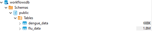
database
Here I connect to the SQL database and inspect the database with the help of R. With the help of “dbConnect” I can load the database in an object called “con”. within this function I need to specify:
dbname: The name of the database
host: where the database is hosted, on my own pc in this case
port: the connection port
user: the username
password: the password, in this example a bad password is used.
with “dbListTables()” I show all tables that are seen (can also be seen in the “database” picture above)
with “dbListField()” I show all fields within “flu_data” in this case
You can also put SQL language in R by using “dbGetQuery()” I used this to show the whole flu_data table. To only show the first 6 rows I put the “head()” function around it.
To disconnect from the database I used the “dbDisconnect()” function
# connect to the database
con <- dbConnect(RPostgres::Postgres(),
                 dbname = "workflowsdb",
                 host="localhost",
                 port="5432",
                 user="postgres",
                 password="kaas")

# laat de tables zien
dbListTables(con)
## [1] "flu_data" "dengue_data" "gapminder"# laat de colummen in flu_data zien
dbListFields(con, "flu_data")## [1] "date" "country" "cases"# laat het tabel flu_data zien
head(dbGetQuery(con, 'SELECT * FROM flu_data'))## date country cases
## 1 Date country cases
## 2 2002-12-29 Argentina NA
## 3 2002-12-29 Australia NA
## 4 2002-12-29 Austria NA
## 5 2002-12-29 Belgium NA
## 6 2002-12-29 Bolivia NA# disconnect van de database
dbDisconnect(con) These are the commands I used in the sql database with the program DBeaver to create the gapminder table. I also used the COPY function again to import the data. And used CONSTRAINT to make a key based on Date and country
#create gapminder table
CREATE TABLE gapminder (
country VARCHAR(50),
Date VARCHAR(50),
infant_mortality VARCHAR(50) not null,
life_expectancy VARCHAR(50) not null,
fertitlity VARCHAR(50) not null,
population VARCHAR(50) not null,
gdp VARCHAR(50) not null,
continent VARCHAR(50),
region VARCHAR(50),
CONSTRAINT PK_gapminder PRIMARY KEY (Date,country)
);
#import the gampinder file
COPY gapminder FROM 'C:/Users/Bas/Desktop/School/Programmeren/datascience/portfolio/data/gapminder_tidy.csv' WITH (FORMAT csv);
# laat de tabel zien
SELECT * FROM gapminder; In the next lines of code I connected to the database again and selected the flu_data and gapminder in one table using the primary key (data, country) I saved this data in “gapminder_flu” and disconnected. gapminder_flu can now be used to create some graphs of the data.
# connect to the database
con <- dbConnect(RPostgres::Postgres(),
dbname = "workflowsdb",
host="localhost",
port="5432",
user="postgres",
password="kaas")
gapminder_flu <- dbGetQuery(con, 'select distinct *
from flu_data,gapminder
where flu_data.country = gapminder.country;'
)
# disconnect van de database
dbDisconnect(con) The first graph that I made are the average amount of flu cases in the Netherlands over time. I did this by first filtering for the country Netherlands. After this I grouped the data by date using the “group_by” function, the date column didn’t have the correct class yet so I used as.Date to make it a Date class. With this dataset I could now calculate the mean amount of cases per data.
I used ggplot with geom_line to create the graph. Where x = date an Y = mean_cases
# filter for the Netherlands and calculate the average cases over time
cases_netherlands <- gapminder_flu %>% filter(country == "Netherlands") %>% group_by(date=as.Date(date)) %>% summarise(mean_cases=mean(as.numeric(cases)))

# make a gg line plot
netherlands_graph <- cases_netherlands %>%
  ggplot(aes(x = date, y = mean_cases)) +
  geom_line() +
  labs(
    title = "Mean flu cases over time in the netherlands",
    y = "cases"
  )
netherlands_graph
In the above graph you can see a few peaks, this is probaply explained by the flu season, where a lot of people get the flu. You can also see that around 2004 they started tracking the amount of flu cases in 2004.
In the next graph I decided to track the mean amount of flu cases in europian countries in 2015 I first had to filter for the year 2015, I did this with the “between()” function inside the “filter()” function. The between function required the first and the last day of the year 2015. After this I grouped the data by country and calculated the mean amount of flu cases.
With this data it was possible to create another ggplot. Within the “geom_bar” function it is important to put “stat =”identity”“, this allows to code to make a bar graph with an y-axis and an x-axis.
I also changed the angle of the country names to be vertical within “theme”, if this was not done the country text would clutter.
# string naar date veranderen
gapminder_flu$date <- as.Date(gapminder_flu$date)

# nieuw object maken waar het gemmidelde cases is berekend in 2015 in europa
country_cases <- gapminder_flu %>% filter(between(date, as.Date("2015-01-01"), as.Date("2015-12-30"))) %>% filter(continent == "Europe") %>% group_by(country) %>% summarise(mean_cases=mean(as.numeric(cases)))

# ggplot maken
graph <-country_cases %>%
  ggplot(aes(x = country, y = mean_cases, fill = country_cases$country)) +
  geom_bar(stat = "identity") +
  theme(axis.text.x = element_text(angle = 90, vjust = 0.5, hjust=1))+
  labs(
    title = "Average flu cases per europian country in 2015"
  )

# ggplot in een plotly veranderen
graph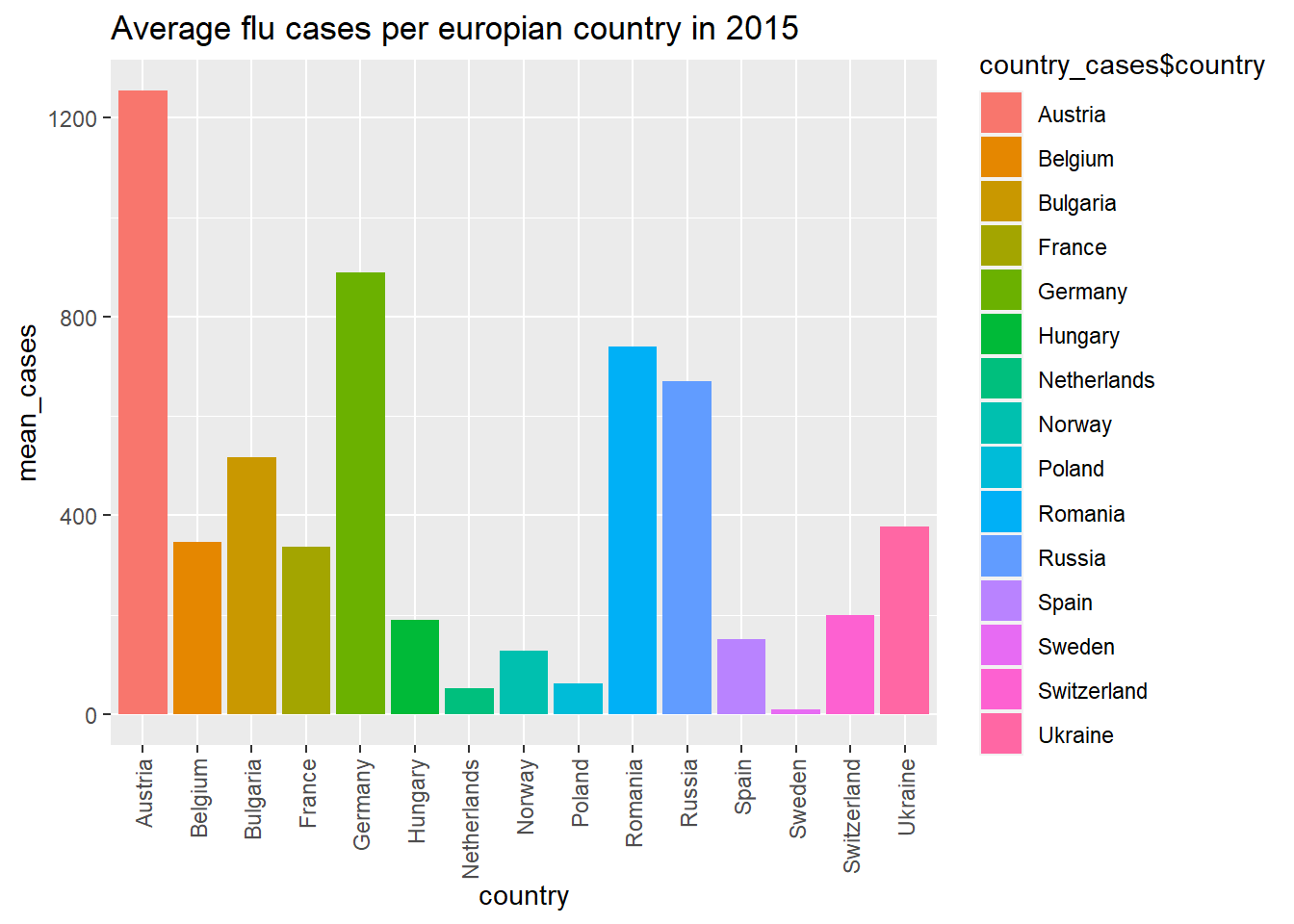
In the above graph you can see Austria had a lot of flu cases in 2015
In the next graph I wanted to plot the average life expectancy per europian country in 2015. I did this with the same filter function as the previous graph expect I calculated the mean life_expactancy after this.
After this I plotted the graph in the same ggplot function.
# string naar date veranderen
gapminder_flu$date <- as.Date(gapminder_flu$date)

# nieuw object maken waar het gemmidelde life_expectancy is berekend in 2015 in europa
country_life <- gapminder_flu %>% filter(between(date, as.Date("2015-01-01"), as.Date("2015-12-30"))) %>% filter(continent == "Europe") %>% group_by(country) %>% summarise(mean_cases=mean(as.numeric(life_expectancy)))

# ggplot maken
graph_life <-country_life %>%
  ggplot(aes(x = country, y = mean_cases, fill = country_cases$country)) +
  geom_bar(stat = "identity") +
  theme(axis.text.x = element_text(angle = 90, vjust = 0.5, hjust=1))+
  labs(
    title = "Average life expectancy per europian country in 2015"
  )

# ggplot in een plotly veranderen
graph_life
In this last graph you can see the life expectancy of a few countries. In Europe the average of lays around 70 years old.