6 Reproducibility

6.1 Working with articles

One of the skills that are useful in datascience is looking at a paper and using the code in the paper to get the exact same result with the dataset. This is call reproducibility.

One of the skills I have learned is to Judge an article based on its reproducibility. To show my skill on juding reproducibiility a grabbed a random article from pubmed you can find this article here

This article looks at the safety of some of the first covid-19 vaccines.

6.1.1 Article References

Edward E. Walsh, M.D., Robert W. Frenck, Jr., M.D., Ann R. Falsey, M.D., Nicholas Kitchin, M.D., Judith Absalon, M.D.,corresponding author Alejandra Gurtman, M.D., Stephen Lockhart, D.M., Kathleen Neuzil, M.D., Mark J. Mulligan, M.D., Ruth Bailey, B.Sc., Kena A. Swanson, Ph.D., Ping Li, Ph.D., Kenneth Koury, Ph.D., Warren Kalina, Ph.D., David Cooper, Ph.D., Camila Fontes-Garfias, B.Sc., Pei-Yong Shi, Ph.D., Özlem Türeci, M.D., Kristin R. Tompkins, B.Sc., Kirsten E. Lyke, M.D., Vanessa Raabe, M.D., Philip R. Dormitzer, M.D., Kathrin U. Jansen, Ph.D., Uğur Şahin, M.D., and William C. Gruber, M.D.

6.1.2 Criteria article

Transparency Criteria	Definition	Response Type	Response type Article
Study Purpose	A concise statement in the introduction of the article, often in the last paragraph, that establishes the reason the research was conducted. Also called the study objective.	Binary	Yes
Data Availability Statement	A statement, in an individual section offset from the main body of text, that explains how or if one can access a study’s data. The title of the section may vary, but it must explicitly mention data; it is therefore distinct from a supplementary materials section.	Binary	Yes
Data Location	Where the article’s data can be accessed, either raw or processed.	Found Value	Email the author
Study Location	Author has stated in the methods section where the study took place or the data’s country/region of origin.	Binary; Found Value	No
Author Review	The professionalism of the contact information that the author has provided in the manuscript.	Found Value	Found by author
information
Ethics Statement	A statement within the manuscript indicating any ethical concerns, including the presence of sensitive data.	Binary	Yes
Funding Statement	A statement within the manuscript indicating whether or not the authors received funding for their research.	Binary	Yes
Code Availability	Authors have shared access to the most updated code that they used in their study, including code used for analysis.	Binary	No

6.1.3 Other data

The protocol, the ethics statement and the data sharing statement are founde beneath the article.

6.1.4 Extra’s about the article

In general this is a good reproducible article that test the safety of multiple covid-19 vaccines with the help of a placebo trial. On of the things that made this article very reproducible is because it is covid-19 related. After the first wave of covid scientist started openly sharing their data to make the best vaccines as soon as possible.

6.2 Working with code from articles

In data science it is also a useful skill to work with open science articles. These articles show their code and show how they got their data. In this part of the page I look at some code and try to reproduce it of a random article. The article is found here

When looking at the code I can see that the data analysts first made some function for the purpose of creating some graphs. After this the load in the required data and look for missing value data. After cleaning the data the started making some graphs.

One of the things that I look at when analysing the code is if the code hase comments describing what is being done in the code. This code has comments above every code but the comment are not always as clear as can be.

After I analysed the code I copied some of the code to look at how easy it is to reproduce the article.

library(here)
# read data ---------------------------------------------------------------
# sample 1
sample1 <- read.csv(here("data","sample1_use for revision 1.csv"))
sample1 <- sample1[sample1$include_1,]

# sample 2
sample2 <- read.csv(here("data","sample2_use for revision 1.csv"))
sample2 <- sample2[sample2$include_1,]

# combine samples for the additional analyses
data <- rbind(sample1, sample2)

# packages ----------------------------------------------------------------
# functie inladen
gg_color_hue <- function(n) {
  hues = seq(15, 375, length = n + 1)
  hcl(h = hues, l = 65, c = 100)[1:n]
}

get_max_daily <- function(x){
  x <- x + c(1:4, 9:12, 17:20, 25:27)
  x <- x[x < ymd("2020-04-13 UTC")]
  return(x)
}

# install.packages("lubridate")
library(lubridate)

# -------------------------------------------------------------------------

## define colors
c <- gg_color_hue(2)
col.s1 <- c[1]
col.s2 <- c[2]

# completed baseline surveys per day that are included in the study
data_l2_s1 <- unique(sample1[c("ID", "b_baseline_ended")])
data_l2_s2 <- unique(sample2[c("ID", "b_baseline_ended")])

# no missings on this variable
any(is.na(data_l2_s1[2]))

## [1] FALSE

any(is.na(data_l2_s2[2]))

## [1] FALSE

date_s1 <- ymd_hms(data_l2_s1$b_baseline_ended)
hour(date_s1) <- 0
minute(date_s1) <- 0
second(date_s1) <- 0

date_s2 <- ymd_hms(data_l2_s2$b_baseline_ended)
hour(date_s2) <- 0
minute(date_s2) <- 0
second(date_s2) <- 0


# number of baseline surveys completed
t_date_baseline_1 <- table(ymd(date_s1))
t_date_baseline_2 <- table(ymd(date_s2))
t_date_baseline_1 <- c(t_date_baseline_1, "2020-04-12" = 0)
t_date_baseline_12 <- rbind(t_date_baseline_1, t_date_baseline_2)

# barplot sample 1 and 2 baseline participation ---------------------------

layout(matrix(1:2, 1, 2, byrow = TRUE))

b <- barplot(t_date_baseline_12, beside = TRUE, ylim = c(0, 800), names.arg = rep("", length(t_date_baseline_12)),
             col = c(col.s1, col.s2), axes = FALSE)
box()
axis(2, las = 2, cex.axis = 0.8)
s <- seq(1, 28, 7)
labels <- colnames(t_date_baseline_12)[s]
axis(1, at = ((b[1,] + b[2,])/2)[s], labels = labels, cex.axis = 0.8)
text("A", x = ((b[1,] + b[2,])/2)[2], y = 800*.9, cex = 4, col = "grey")
legend(x = ((b[1,] + b[2,])/2)[15], y = 800, legend = c("Sample 1", "Sample 2"), fill = c(col.s1, col.s2), bty = "n")


# dates at which a daily survey could have been completed:
max_daily_dates_s1 <- lapply(ymd(date_s1), get_max_daily)
max_daily_dates_s2 <- lapply(ymd(date_s2), get_max_daily)

max_dates_s1 <- do.call("c", max_daily_dates_s1)
max_dates_s2 <- do.call("c", max_daily_dates_s2)
obtained_dates_s1 <- sample1$daily_date
obtained_dates_s2 <- sample2$daily_date

t_max_dates_s1 <- table(max_dates_s1)
t_max_dates_s2 <- table(max_dates_s2)

t_obtained_dates_s1 <- table(obtained_dates_s1)
t_obtained_dates_s2 <- table(obtained_dates_s2)

t_obtained_dates_s12 <- rbind(t_obtained_dates_s1, t_obtained_dates_s2)

b <- barplot(t_obtained_dates_s12, beside = TRUE, ylim = c(0, 2000),
             names.arg = rep("", length(t_obtained_dates_s12)),
             col = c(col.s1, col.s2), axes = FALSE)
box()
axis(2, las = 2, cex.axis = 0.8)
labels <- colnames(t_obtained_dates_s12)[s]
axis(1, at = ((b[1,] + b[2,])/2)[s], labels = labels, cex.axis = 0.8)

lines(y = t_max_dates_s1, x = b[1,], type = "p", pch = "-", col = col.s1, cex = 1.5)
lines(y = t_max_dates_s2, x = b[2,], type = "p", pch = "-", col = col.s2, cex = 1.5)
text("B", x = ((b[1,] + b[2,])/2)[2], y = 2000*.9, cex = 4, col = "grey")
legend(x = ((b[1,] + b[2,])/2)[15], y = 2000, legend = c("Sample 1", "Sample 2"), fill = c(col.s1, col.s2), bty = "n")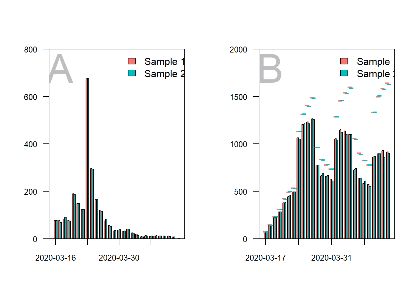

# difference obtained and maximum -----------------------------------------

obtained_total <- sum(t_obtained_dates_s12)
max_reports_total <- sum(c(t_max_dates_s1, t_max_dates_s2))
round(obtained_total/max_reports_total*100, 2)

## [1] 75.74

# average surveys per day -------------------------------------------------

median(colSums(t_obtained_dates_s12))

## [1] 1468

# average number of loneliness scores per participant ---------------------

s1_lst <- split(sample1, f = sample1$ID)
n_1 <- unlist(lapply(s1_lst, function(x) sum(!is.na(x$loneliness))))
mean(n_1)

## [1] 8.150741

sd(n_1)

## [1] 3.359446

range(n_1)

## [1]  0 15

s2_lst <- split(sample2, f = sample2$ID)
n_2 <- unlist(lapply(s2_lst, function(x) sum(!is.na(x$loneliness))))
mean(n_2)

## [1] 8.124586

sd(n_2)

## [1] 3.399153

range(n_2)

## [1]  0 15

# distribution of participants across number of daily surveys
layout(1)
b <- barplot(table(c(n_1, n_2)), main = "", ylab = "valid loneliness scores",
             xlab = "number of completed daily surveys",
             ylim = c(0, 900), lwd = 1.3)
box(lwd = 1.3)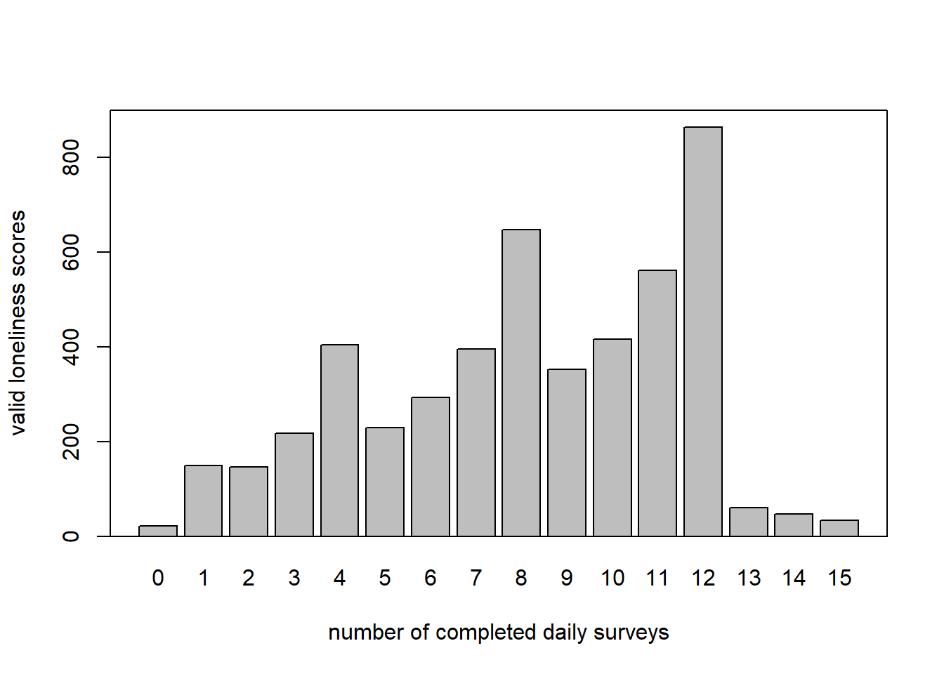

# surveys, not valid measures
n_1 <- unlist(lapply(s1_lst, function(x) nrow(x)))
n_2 <- unlist(lapply(s2_lst, function(x) nrow(x)))
mean(n_1)

## [1] 8.269769

sd(n_1)

## [1] 3.318693

range(n_1)

## [1]  1 15

mean(n_2)

## [1] 8.25207

sd(n_2)

## [1] 3.359575

range(n_2)

## [1]  1 15

b <- barplot(table(c(n_1, n_2)), main = "", ylab = "N",
             xlab = "number of completed daily surveys",
             ylim = c(0, 1000), lwd = 1.3)
box(lwd = 1.3)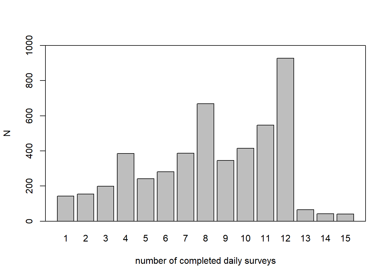

# N and measurement occasions ---------------------------------------------

sample1_lst <- split(sample1, f = sample1$ID)
sample2_lst <- split(sample2, f = sample2$ID)

length(sample1_lst)

## [1] 2428

length(sample2_lst)

## [1] 2416

length(sample1_lst) + length(sample2_lst)

## [1] 4844

nrow(sample1)

## [1] 20079

nrow(sample2)

## [1] 19937

nrow(sample1) + nrow(sample2)

## [1] 40016

# demographic variables ---------------------------------------------------

names <- names(sample1)
variables_level_2 <- grep(x = names, pattern = "ID|group|b_|var_|federal", value = TRUE)
data_l2_s1 <- unique(sample1[variables_level_2])
data_l2_s2 <- unique(sample2[variables_level_2])

## age
mean(data_l2_s1$b_demo_age_1)

## [1] 37.29462

sd(data_l2_s1$b_demo_age_1)

## [1] 14.32523

mean(data_l2_s2$b_demo_age_1)

## [1] 37.57201

sd(data_l2_s2$b_demo_age_1)

## [1] 14.24426

# generate level 2 data frame for all participants
data_l2 <- unique(data[c(grep(x = names(data), pattern = "ID|b_demo|b_work|b_corona", value = TRUE))])

mean(data_l2$b_demo_age_1)

## [1] 37.87923

sd(data_l2$b_demo_age_1)

## [1] 14.40773

barplot(table(data_l2$b_demo_age_1), main = "Distribution of age across the total sample", lwd = 1.3, ylim = c(0, 200))
box(lwd = 1.3)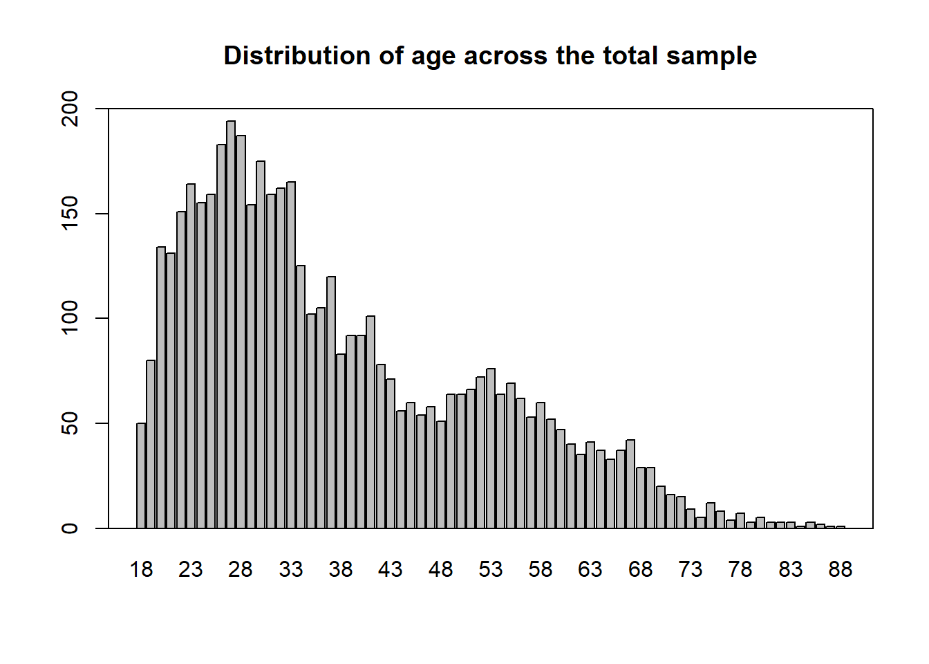

## quartiles of age
quantile(data_l2$b_demo_age_1)

##   0%  25%  50%  75% 100% 
##   18   27   34   48   88

There are a few things I had to change within the code:

• I had to change the path the data was led to

• Some functions where loaded in another file, I copied them to the code, the functions were: “gg_color_hue” and “get_max_daily”

One of the things with the output of the graphs is that they don’t contain y-axis descriptions. This article was pretty easy to reproduce the code only needed a few changes. To rate the article on reproducible I would rate it about a four on a scale of one to five.